Closure phase

The closure phase is an observable quantity in imaging astronomical interferometry, which allowed the use of interferometry with very long baselines. It forms the basis of the self-calibration approach to interferometric imaging. The observable which is usually used in most "closure phase" observations is actually the complex quantity called the triple product (or bispectrum). The closure phase is the phase of this complex quantity, but the phrase "closure phase" is still more commonly used than the more accurate phrase "triple product".

Roger Jennison developed this novel technique for obtaining information about visibility phases in an interferometer when delay errors are present. Although his initial laboratory measurements of closure phase had been done at optical wavelengths, he foresaw greater potential for his technique in radio interferometry. In 1958 he demonstrated its effectiveness with a radio interferometer, but it only became widely used for long baseline radio interferometry in 1974. A minimum of three antennas are required. This method was used for the first VLBI measurements, and a modified form of this approach ("Self-Calibration") is still used today. The "closure-phase" or "self-calibration" methods are also used to eliminate the effects of astronomical seeing in optical and infrared observations using astronomical interferometers.

Definition

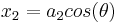
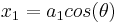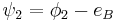
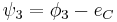
A minimum of three antennas are required for closure phase measurements. In the simplest case, with three antennas in a line separated by the distances a₁ and a₂ shown in diagram at the right. The radio signals received are recorded onto magnetic tapes and sent to a laboratory as described in the article on Very Long Baseline Interferometry. The effective baselines for a source at an angle $\theta$ will be $x_{1}=a_{1}cos(\theta)$ , $x_{2}=a_{2}cos(\theta)$ and $x_{3}=(a_{1}%2Ba_{2})cos(\theta)$ . 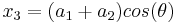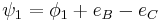The phases of the complex visibility of the radio source corresponding to baselines x₁, x₂ and x₃ are denoted by $\phi_{1}$ , $\phi_{2}$ and $\phi_{3}$ respectively. The phase of interference fringes on each baseline will contain errors resulting from e_B and e_C in the signal phases. The measured phases for baselines x₁, x₂ and x₃, denoted $\psi_{1}$ , $\psi_{2}$ and $\psi_{3}$ , will be:

$\psi_{1}= \phi_{1}%2Be_{B}-e_{C}$

$\psi_{2}= \phi_{2}-e_{B}$

$\psi_{3}= \phi_{3}-e_{C}$

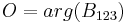
Jennison defined his observable O (now called the closure phase) for the three antennas as:

$O = \psi_{1}%2B \psi_{2}- \psi_{3}$

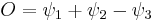
As the error terms cancel:

$O = \phi_{1}%2B \phi_{2}- \phi_{3}$

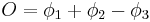
The closure phase is unaffected by phase errors at any of the antennas. Because of this property, it is widely used for aperture synthesis imaging in astronomical interferometry. In most real observations, the complex visibilities are actually multiplied together to form the triple product instead of simply summing the visibility phases. The phase of the triple product is the closure phase.

In optical interferometry, the closure phase was first introduced by the bispectrum speckle interferometry (Reference?). There was a long debate as to whether it was strictly equivalent to the radio closure phase until (Reference?). The principle is to compute the closure phase from the complex measurement instead of the phase itself:

$B_{123}= C_{12} C_{23} C_{13}^{*}$

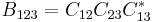
The closure phase is then computed as the argument of this bispectrum:

$O = arg(B_{123})$

This method of computation is robust to noise and allow to perform averaging even if the noise dominates the phase signal.

References

Roger Jennison, A phase sensitive interferometer technique for the measurement of the Fourier transforms of spatial brightness distributions of small angular extent, Monthly Notices of the Royal Astronomical Society vol 118 pp 276 1958

Roger Jennison, The Michelson stellar interferometer : a phase sensitive variation of the optical instrument, Proc. Phys. Soc. 78, 596–599, 1961.